Running and reviewing static analysis in Robot
Any referenced datasets can be downloaded from "Module downloads" in the module overview.
Running and reviewing static analysis in Robot - Exercise
In this practice, you will step through the process of running finite element analysis in Robot and displaying results as diagrams on bars, maps on panels, and text output in tables.
- Open Autodesk Robot Structural Analysis Professional 2020.
- Open in it the project STRUCTURAL_before design.rtd.
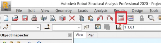
- Select the Calculations icon marked below to run analysis.
- Accept the message about separate structure displayed during analysis and close the Calculation Massages window displayed after analysis. Pay attention to the Results (FEM): available status message displayed in the title bar, after the name of the model, and in the status bar, at the bottom of the screen.
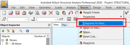
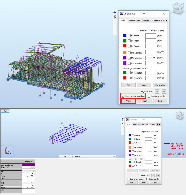
- Select Results > Diagrams for Bars… from the pull-down text menu.
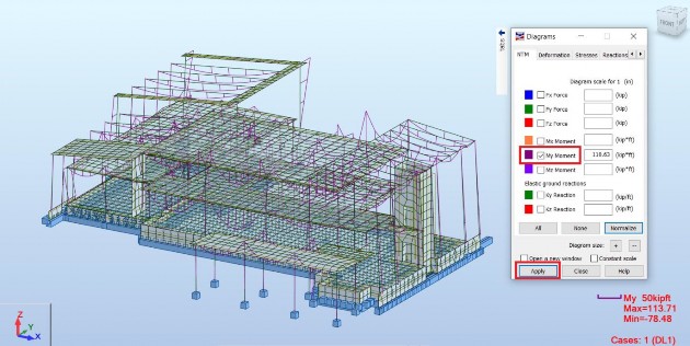
- Activate the My Moment in the Diagrams dialog box and select Apply to display My diagrams on bars for the whole model for the active load case.
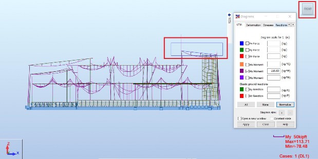
- Click the FRONT face of the View Cube to set a front view of the model and select graphically by rectangle (dragging the mouse cursor from left to right) the bars on the roof of the model on the right side, as shown below.
- Return to the default 3D view by moving mouse cursor over the View Cube and clicking the home icon when it is displayed.

- Activate Open a new window in the Diagrams dialog box and select Apply to open a new graphic window with the previously selected part of the model.
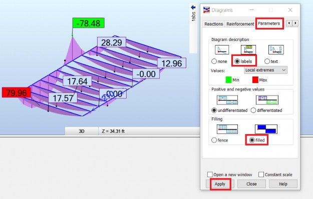
- In the Parameters tab of the Diagrams dialog box, activate labels and filled and select Apply to display filled diagrams with descriptions.
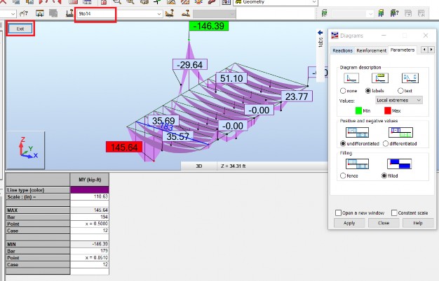
- Click the field of load case selection marked below, input the list of cases 9to14 and press Enter on the keyboard to accept. The envelope of My moments for ULS combinations 9to14 will be displayed. Then select the Exit button, marked below, to close the additional Diagrams viewer and return to the main View.
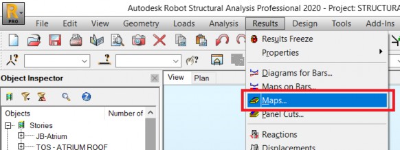
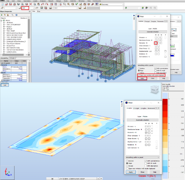
- Select Results > Maps… from the pull-down text menu.
- Click the field of bar and panel selection marked below, input the number of panel 224 and press Enter on the keyboard to accept. The panel highlighted below in blue will be selected. Activate Moments - M for xx, activate Open a new window in Maps dialog box and select Apply to open a new graphic window with maps of MXX moments for the previously selected panel.
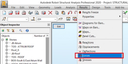
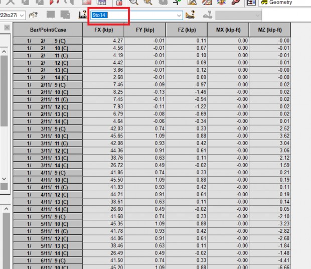
- Select Results > Forces from the pull-down text menu.
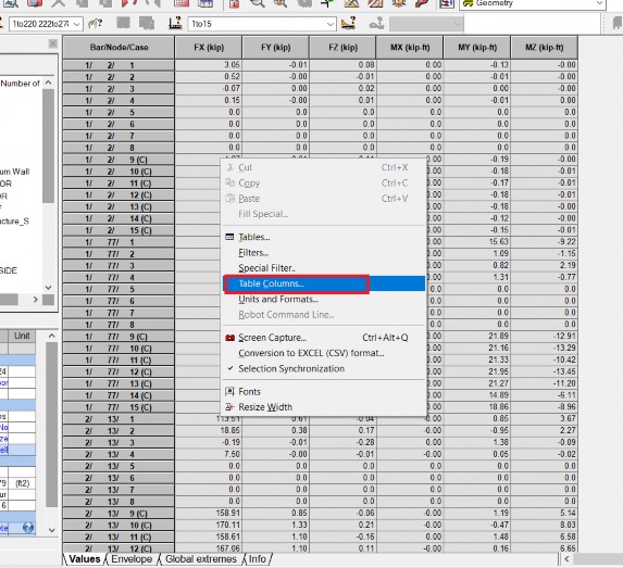
- Click the right mouse button over the displayed map of forces to display the context-menu. Select Table Columns… from it.
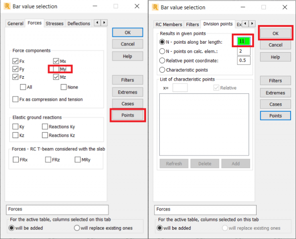
- The Bar value selection dialog box is displayed. Switch off the display of My moment in it and select the Points button or switch to the Division points tab of the dialog box. Change the number of points from 2 to 11 and select OK.
- Click the field of load case filtering marked below, input the list of cases 9to14, and press Enter on the keyboard to accept. The contents of the table will be filtered to show only ULS combinations.
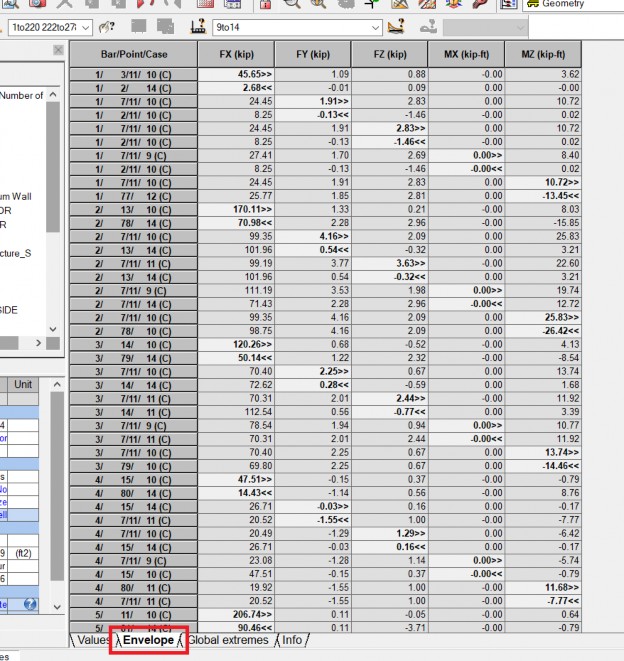
- Select the Envelope tab of the table to display the extreme values of forces and moments for each bar for the currently filtered list of load cases and combinations.
- Save the model with a new name using File > Save As… from the pull-down text menu.