Importing and validating Point Cloud data

Importing and validating Point Cloud data - Exercise

Task 1: Begin a new drawing in Civil 3D

1. Launch Civil 3D using the Metric shortcut. This will start a new drawing named Drawing 1. If you want to save it, you will have to give it a folder location and a name.
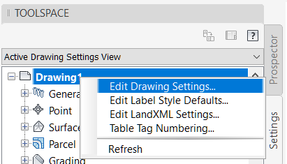
2. On the Settings tab of the Toolspace, hover over the drawing name at the top of the collections tree and right-click.
3. Select Edit Drawing Settings.
   
   
   
   
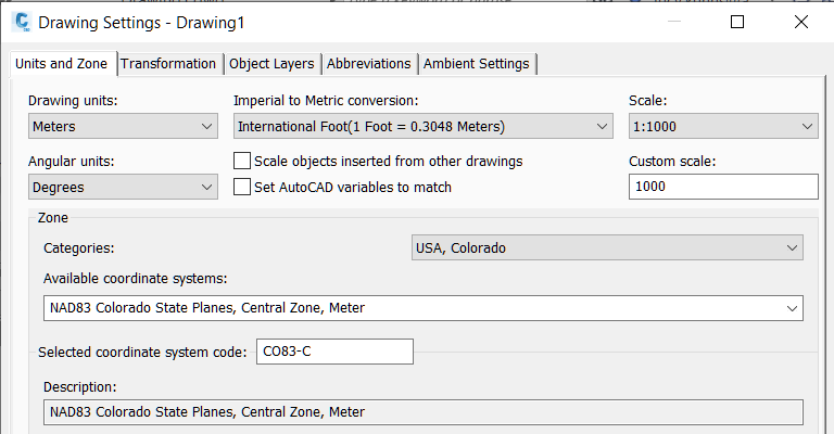
4. On the Units and Zone tab, verify that the units are Meters.
5. In the Zone category, drop down the list and select: USA, Colorado.
6. Drop down the list of available coordinate systems and select: NAD83 Colorado State Planes, Central Zone, Meter.
7. Verify that the Selected coordinate system code is: CO83-C.
8. Click OK.
   
   

Task 2: Attach Point Cloud

1. On the Insert tab, click on the Attach Point Cloud icon.
   
   
   
   
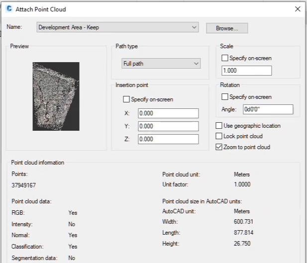
2. Browse to the exercise data set and select the file Development Area – Keep.rcs.
3. On the Attach Point Cloud Dialog box, click on Details.
4. Verify the number of points in the point cloud.
5. Review the other point cloud data to see that it is RGB and Classified.
   
   
   
   
6. When the point cloud is attached the view style changes to 3D Wireframe so the point cloud is displayed. Point cloud data does not display in 2D view styles.

Task 3: Set 3D Osnap

1. Select the Osnap icon in the Civil 3D tray, or type in OSNAP.
2. Select the 3D Osnap tab.
3. In the Point Cloud list, toggle on Node.
4. Place a checkmark in the 3D Object Snap On box.
   
   
   
   
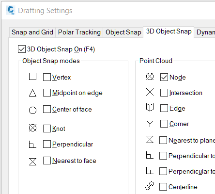
5. Click OK.

Task 4: Check size and units

1. Zoom to the main intersection area.
   
   
   
   
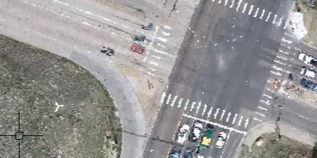
2. Notice the white triangular panel point marking seen to the southwest side of the intersection.
3. Zoom in closer to see the white lane markings between the automobiles.
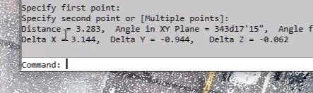
4. Use the Distance command to pick two points to measure the distance between the white stripes.
   
   
   
   
5. Use the F2 key to open the command line history so that you can see the length measurement.
6. Verify that the distance is almost 3.2 meters.
   
   
   
   
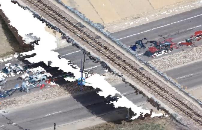
7. Navigate to the railroad bridge and check the distance between the bridge deck and the top of the pavement. This distance should be about 6.8 meters.
   
   

Task 5: Crop a small area of interest

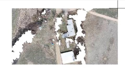
1. Navigate to the area around the house and barn buildings in the southern part of the project.
2. Turn off 3D Osnap. Tip: use F4 to toggle.
3. Select on the boundary of the point cloud so that the context sensitive ribbon is displayed. Tip: try a crossing window selection.
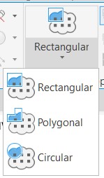
4. On the Cropping ribbon panel, click on Rectangular.
   
   
   
   
5. Pick two points to define the area of interest.
   
   
   
   
6. Right-click and select Inside to keep the points that are inside this cropping rectangle.

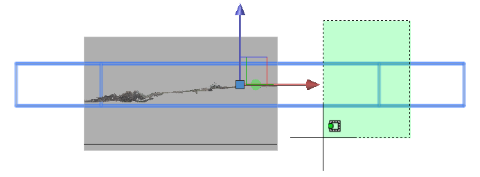
Task 6: Create and view a sliced section

1. Select the point cloud to display the context ribbon.
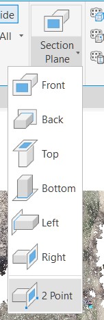
2. On the Section ribbon panel, click on 2 Point.
   
   
   
   
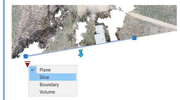
3. Pick two points that cut across an interesting part of the data – for example, from the pond area through one of the buildings.
4. Click on the dropdown glyph and select Slice.
   
   
   
   
5. Use the sizing arrow grips to make the slice narrow.
   
   
   
   
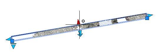
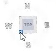
6. Use the Nav Cube to get a SW view.
   
   
   
   
7. Select on one of the long edge of section lines to display the glyphs and grips.
8. Select on the 3D gizmo and then on the Z axis.
9. Slide up along the Z axis to raise the system to a position just under the point cloud.
   
   
   
   
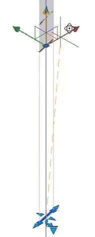
10. Use the height of limits box arrow to lower the upper limit to a position near the top of the point cloud data. Moving the upper and lower limits gives an easier to use sliced section.
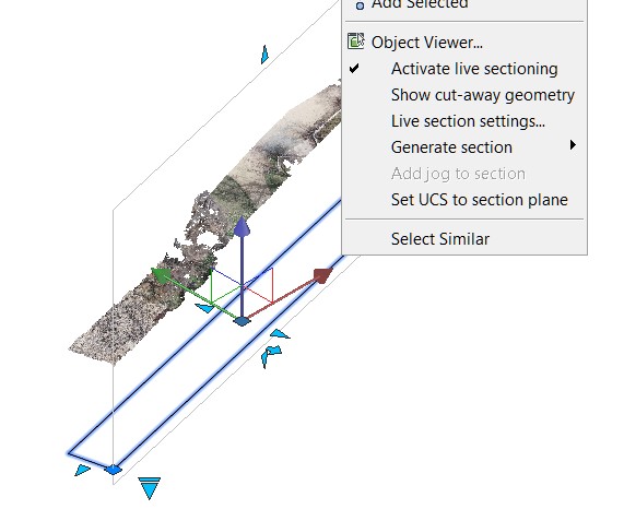
11. Select on the rectangle at the base of the section and right click to access the pop-up menu.
12. Click on Set UCS to section plane.
    
    
    
    
13. At the command line, type in PLAN.
14. Accept the default option Current.
15. Pan and zoom to the section view.

Task 7: Review classification in Section view

1. Select the point cloud boundary. Tip: Use a crossing window in a blank are just outside the slice.
   
   
   
   
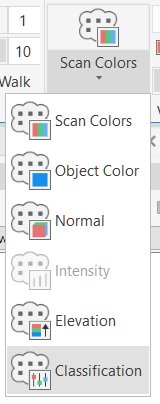
2. In the context ribbon, select Classification in the Visualization panel.
   
   
   
   
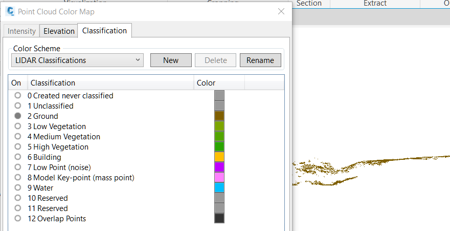
3. Click on Color Mapping to open the classification color mapping.
4. Use shift select to select all classifications, pick on one on button to turn off the display of all colors. Click Apply.
5. Experiment with turning on and off the different classifications to see how they influence the ground surface representation. Make sure to click Apply to see the changes.
   
   
   
   
6. Return to the World UCS. Enter in UCS at the command line and select the World option.
7. Enter PLAN at the command line and select the Current option. This will place the point cloud in a top view.
8. Select on the edge of the section rectangle and erase or delete it. This will return to the cropped point cloud.
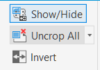
9. Select the point cloud and in the Cropping pane, click Uncrop All.
   
   
   
   
10. This drawing will be used in the next objective exercise.