Identify 2D sediment transport equations

Step-by-step guide

In InfoWorks ICM, empirical equations are used to simulate 2D sediment transport in rivers.

The QM Parameters and the Water quality and sediment parameters are used to apply different equations that model suspended sediment and bed load transport in 2D.

To set the simulation parameters:

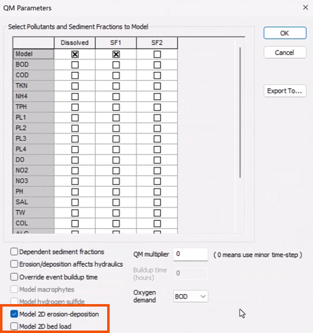
1. In the Run dialog, select QM parameters.

2. In the QM Parameters dialog, select either:

• Model 2D erosion-deposition to simulate both bed and suspended sediment loads.
• Model 2D bed load to simulate bed load transport only.

To set the water quality parameters:

3. Select Model > Model parameters > Water quality and sediment parameters.
4. In the Properties panel, select a Model type.

• Suspended load models only the suspended load.
• Total load models the total sediment load, including the suspended load and the bed load.
• Bed load models only the bed load.

It is important to keep the following in mind:

• If the Model type is set to Total load, verify that only one option is selected in QM Parameters. Selecting both will cause double counting of bed load transport and will result in simulation failure.
• If Model 2D bed load is selected in QM Parameters, the only available Model type will be Bed load transport. Simulating suspended sediment is not possible with this option.

The table below shows the various combinations of parameters and the result of each:

Water quality parameters	Simulation parameters	Result
Suspended load	Model 2D erosion-deposition	Suspended material only
Total load	Model 2D erosion-deposition	Both suspended and bed load
Bed load	Model 2D bed load	Bed load
Suspended load (N/A)	Model 2D bed load	Not possible

Suspended load model

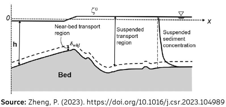
Remember that Suspended load is the suspension of fine particles, such as silt and clay, within the mass of fluid.

For the 2D erosion/deposition model, if the Model type is set to Suspended load, three additional options become available for selecting the corresponding equations.

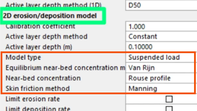
• Near-bed concentration is the concentration of particles in the fluid closest to the bed of a river.
• Skin friction is the resistance caused by fluid viscosity.
• Equilibrium near-bed concentration is the state where particle concentration near the bed remains constant over time. This occurs when the rate of particle deposition onto the bed is equal to the rate of resuspension into the water column.

For Near-bed concentration, two equations are available:

• The Rouse profile approximation describes the vertical distribution of suspended sediment concentration and considers the balance between upward turbulent diffusion and downward settling of particles.
• The Lin formulation models the vertical concentration profile and considers specific flow and sediment characteristics for a more tailored concentration distribution.

For Equilibrium near-bed concentration, the available equations are Van Rijn, Zyserman and Fredsoe, and Smith and McLean. The Van Rijn equation, for example, estimates the reference concentration based on sediment size, flow velocity, and bed shear stress.

For Skin friction, available equations are based on experimental tests.

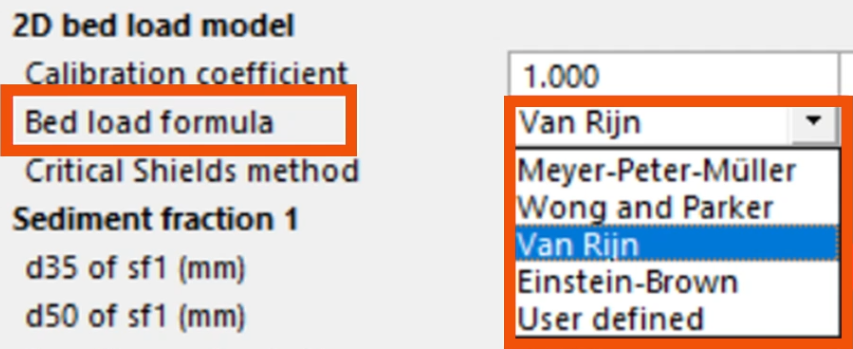
Bed load model

Several equations are available to calculate the carrying capacity of the flow as a volumetric transport rate.

5. In Properties, under 2D bed load model, expand the Bed load formula drop-down.
6. Select an equation. For example, Meyer-Peter-Müller is typically selected for sand and fine gravel bed material.

Total load model

To accurately simulate sediment transport dynamics, it is crucial to select the appropriate equation.

7. In Properties, under 2D erosion/deposition model, expand the Total load model drop-down to select from the available options: Ackers-White, Engelund-Hansen, Westrich-Jurashek, Van Rijn, and Velikanov.

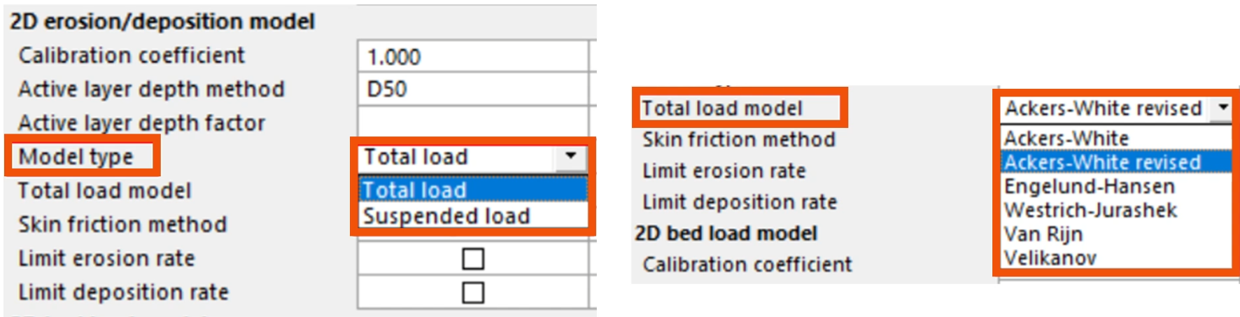
Each equation has specific applications based on sediment type, flow conditions, and environmental settings. For example, Van Rijn is a versatile equation that predicts sediment transport rates, including bed load and suspended load in rivers, accounting for sediment size, flow depth, and current velocity.

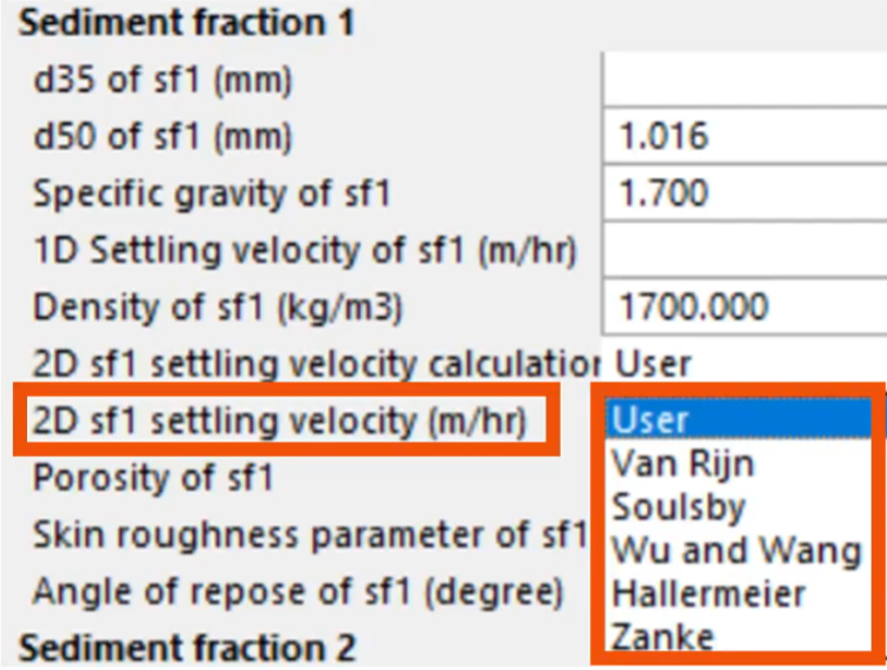
Settling velocity

This is the terminal velocity at which a particle in still fluid ceases to accelerate as the forces acting on it are balanced.

8. In Properties, under Sediment fraction 1, expand the drop-down for 2D sf1 settling velocity (m/hr).
9. Choose from the available formulas: Van Rijn, Soulsby, Wu and Wang, Hallermeier, and Zanke.

Key parameters required for these calculations include particle size, D35, D50, specific gravity, density, porosity, skin roughness, and the angle of repose for sediment.

Next, in ICM, perform a suspended load and total bed load simulation:

10. In the Scenarios drop-down, select Suspended.
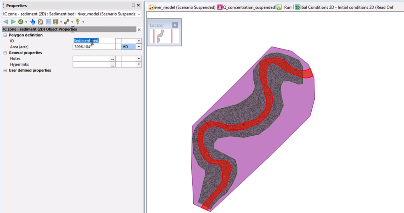
11. On the GeoPlan, select the bed channel.
12. In the Multiple Selection pop-up, select Sediment bed.
13. Click OK.

This is a polygon, where different types of bed material and the concentration of each layer can be defined.

14. In the Explorer, right-click Initial conditions 2D and select Open.
15. In the Variable column, set the value to Bed sediment.
16. Define the type of bed layer and the depth, as well as the concentration layer.
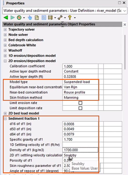
17. Select Model > Model parameters > Water quality and sediment parameters.
18. In Properties, under 2D erosion/deposition model, set the Model type to Suspended load.

For this example, based on the characteristics of the particles in the bed, set the following parameters:

19. Set the Equilibrium near-bed concentration method to Van Rijn.
20. Set Near-bed concentration to Rouse profile.
21. Set the Skin friction method to Manning.
22. Under Sediment fraction 1, specify the size of the particle, Specific gravity, Settling velocity, and other relevant properties.

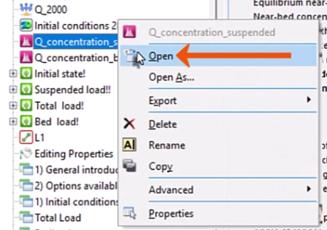
23. From the Explorer, open a pollutograph. In this case, a previously created pollutograph named Q_concentration_suspended is opened.

24. On the SF1 tab, define the variation of particle concentration over time.
25. Right-click one of the profiles and select Profile properties.
26. In the Profile Properties dialog, for Profile type, select Suspended.
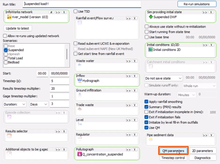
27. Open the Run dialog for the Suspended load run and drag in the pollutograph.
28. Select Use QM.
29. Click QM parameters.

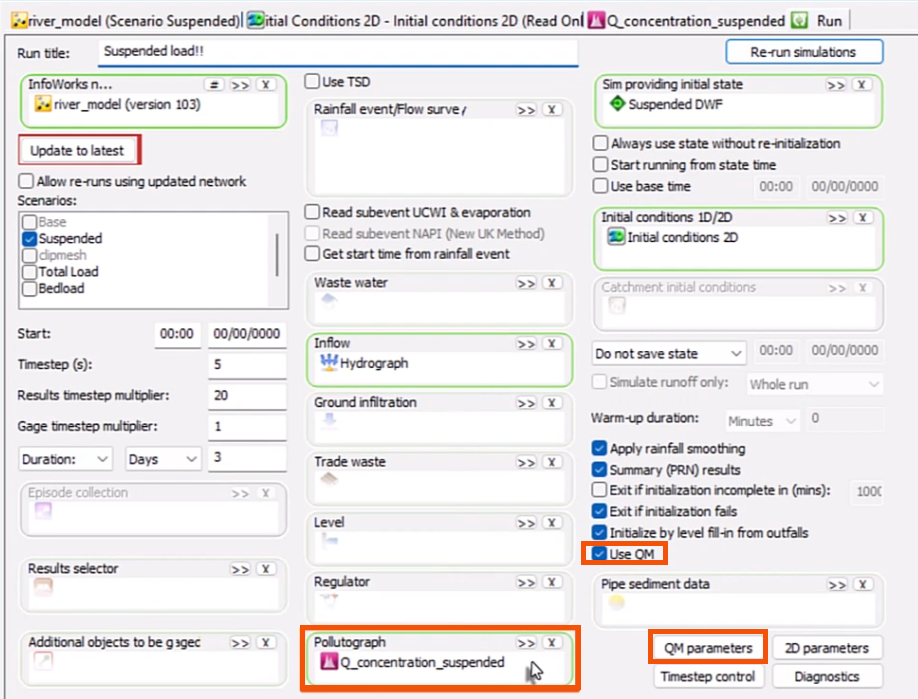
30. In the QM Parameters dialog, select SF1.
31. Verify that Model 2D erosion-deposition is selected.

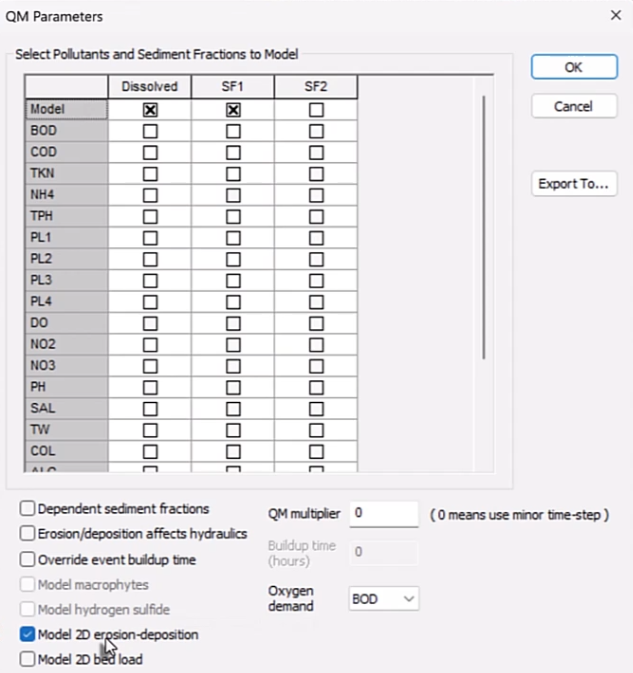
This will perform a suspended load and total bed load simulation. To simulate only bed load, select Model 2D bed load instead.

32. Click OK.
33. Back in the Run dialog, click Run simulations.
34. Confirm the selections in the Schedule Jobs dialog and click OK.
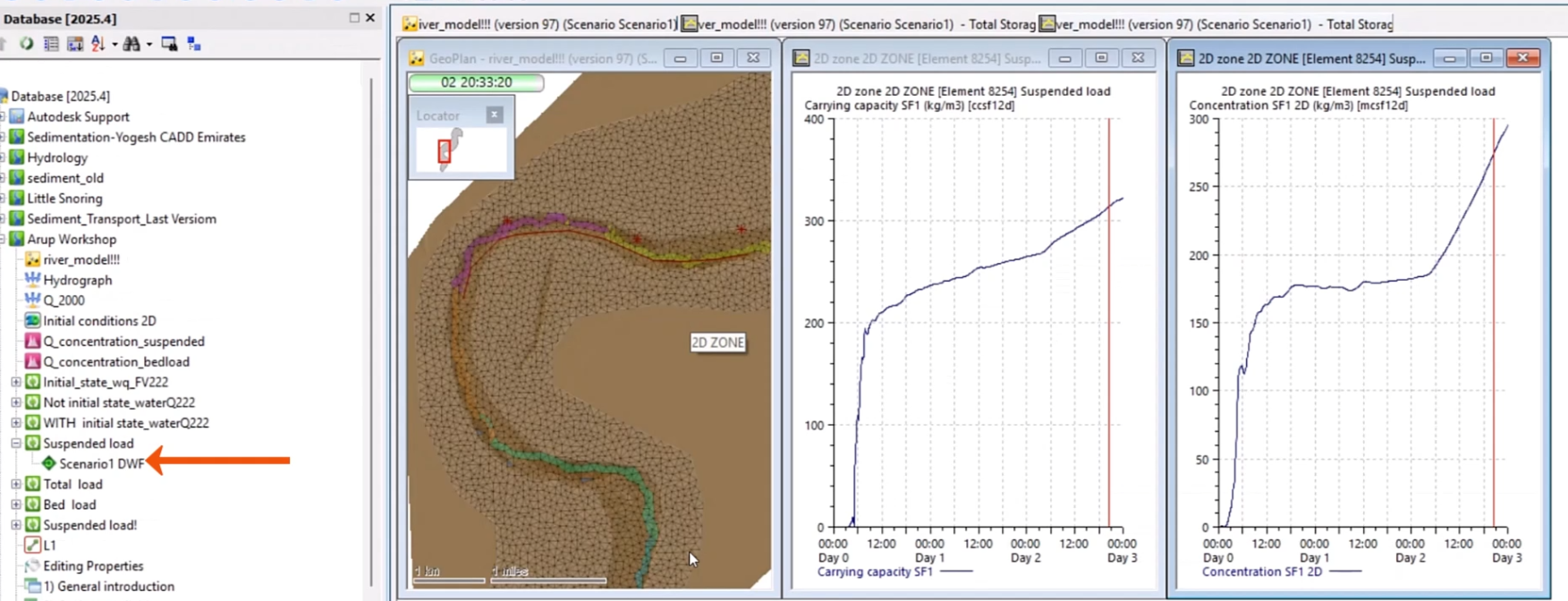
35. In the Explorer, right-click the Suspended load result and select Open to display the plan view and two graphs.

• The plan view shows a thematic map of the distribution of the carrying capacity values along the river reach.
• The first graph shows that the values of carrying capacity are increased in one point close to the meander section.
• The second graph shows suspended concentration at the same point where the carrying capacity was plotted.