Setting up the Multi Solute Water Quality Object

00:03

Multi Solute Water Quality (MSQ) allows you to model several interacting chemicals in the water system.

00:11

In this tutorial, the goal is to model Contaminant A and Contaminant B,

00:16

which then react to produce Contaminant C within the distribution network.

00:20

When using this module for your own work, you will need to have the set of equations to implement already available.

00:28

You will also need to have done your own research as to how to model complex interactions between solutes.

00:35

First, create a new Solute Data Group object.

00:39

From the Model Group, right-click the MSQ Model Group and select New > Solute Group.

00:46

Then, right-click the new Solute Data Group you just created and select New > Solute Data.

00:52

In the popup, name the new solute data object “MSQ Example”.

00:57

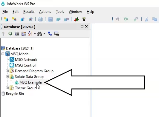
In the Model Group, double-click the MSQ Example solute object to open it.
01:04

In the bottom left of the Solute Data dialog box, deselect the Enable Basic water quality option to turn it off,

01:11

and then select Enable MSQ to allow the MSQ tabs in this dialog to become active.

01:17

In the MSQ Solutes tab, any number of solutes are defined.

01:22

You will populate the first row for Contaminant A, the second row for Contaminant B, and the third row for Contaminant C.

01:30

In the first row, specify the WQ Solute ID as A.

01:34

The solute IDs are used in property sheets and in the results.

01:39

All IDs must be unique within this grid.

01:43

Also set the WQ Solute Description as A.

01:47

In the second row, specify the WQ Solute ID as B and the WQ Solute Description as B.

01:56

Specify the third WQ Solute ID as C and the WQ Solute Description as C.

02:03

For all the rows, from the Solute Type drop-down list, select Bulk (dissolved) to specify that the solute is present in the bulk liquid,

02:12

rather than on the pipe walls.

02:14

Leave the Initial Concentration for Unset Links and Nodes set to zero for A, B, and C.

02:21

In the MSQ Constants tab, constants are used to make equations easier to read but are optional.

02:28

Any number of constant IDs can be defined with associated numerical values.

02:34

The constant IDs are replaced by the numerical values when the engine acts upon the equations.

02:40

Again, you will populate the first row for Contaminant A, the second row for Contaminant B,

02:46

and the third row for Contaminant C.

02:49

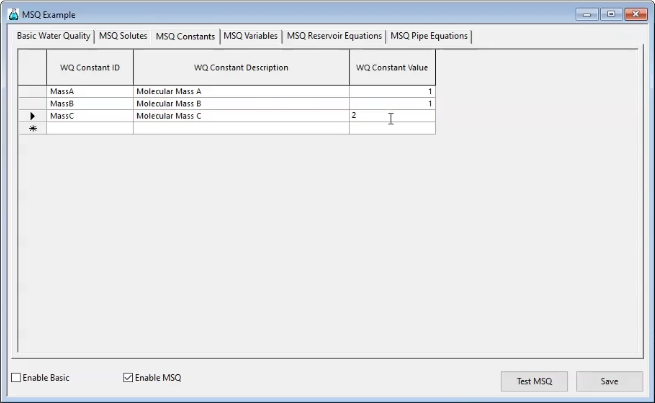
In the first row, specify the WQ Constant ID as Mass A, the WQ Constant Description as Molecular Mass A

02:58

and the WQ Constant Value as 1.

03:01

In the second row, specify the WQ Constant ID as Mass B, the WQ Constant Description as Molecular Mass B

03:09

and the WQ Constant Value as 1.

03:13

In the third row, specify the WQ Constant ID as Mass C, the WQ Constant Description as Molecular Mass C

03:22

and the WQ Constant Value as 2.

03:26

The MSQ Variables tab defines the Variable IDs, one per line in the text editor.

03:32

Variables define an expression by combining constants, numerical values, algebraic operators, and reserved keywords.

03:41

The MSQ Reservoir Equations tab defines the way that solutes change over time within reservoirs.

03:47

One solute is defined per line in this text box.

03:52

Only dissolved (bulk) solutes are considered in this section.

03:56

The equation for each solute is composed of numbers, arithmetic operators, constants, variables, and solute IDs.

04:05

Similarly, in the MSQ Pipe Equations tab, the way that solutes change over time in pipes is defined.

04:13

This deals with changes to adsorbed solutes, as well as those dissolved in the bulk of the water.

04:19

The construction of equations for Pipes follows the same rules as for reservoirs.

04:24

The exception is that pipe equations can also include adsorbed solutes.

04:30

In the MSQ Variables, MSQ Reservoir Equations,

04:35

and MSQ Pipe Equations tabs, copy and paste the scripts provided in the MSQ_Variable.txt, MSQ_Reservoir_Equations.txt

04:44

and MSQ_Pipe_Equations.txt files, respectively.

04:49

When you are finished, click Test MSQ to ensure that there are no errors.

04:56

Click Save.

Video transcript

00:03

Multi Solute Water Quality (MSQ) allows you to model several interacting chemicals in the water system.

00:11

In this tutorial, the goal is to model Contaminant A and Contaminant B,

00:16

which then react to produce Contaminant C within the distribution network.

00:20

When using this module for your own work, you will need to have the set of equations to implement already available.

00:28

You will also need to have done your own research as to how to model complex interactions between solutes.

00:35

First, create a new Solute Data Group object.

00:39

From the Model Group, right-click the MSQ Model Group and select New > Solute Group.

00:46

Then, right-click the new Solute Data Group you just created and select New > Solute Data.

00:52

In the popup, name the new solute data object “MSQ Example”.

00:57

In the Model Group, double-click the MSQ Example solute object to open it.

01:04

In the bottom left of the Solute Data dialog box, deselect the Enable Basic water quality option to turn it off,

01:11

and then select Enable MSQ to allow the MSQ tabs in this dialog to become active.

01:17

In the MSQ Solutes tab, any number of solutes are defined.

01:22

You will populate the first row for Contaminant A, the second row for Contaminant B, and the third row for Contaminant C.

01:30

In the first row, specify the WQ Solute ID as A.

01:34

The solute IDs are used in property sheets and in the results.

01:39

All IDs must be unique within this grid.

01:43

Also set the WQ Solute Description as A.

01:47

In the second row, specify the WQ Solute ID as B and the WQ Solute Description as B.

01:56

Specify the third WQ Solute ID as C and the WQ Solute Description as C.

02:03

For all the rows, from the Solute Type drop-down list, select Bulk (dissolved) to specify that the solute is present in the bulk liquid,

02:12

rather than on the pipe walls.

02:14

Leave the Initial Concentration for Unset Links and Nodes set to zero for A, B, and C.

02:21

In the MSQ Constants tab, constants are used to make equations easier to read but are optional.

02:28

Any number of constant IDs can be defined with associated numerical values.

02:34

The constant IDs are replaced by the numerical values when the engine acts upon the equations.

02:40

Again, you will populate the first row for Contaminant A, the second row for Contaminant B,

02:46

and the third row for Contaminant C.

02:49

In the first row, specify the WQ Constant ID as Mass A, the WQ Constant Description as Molecular Mass A

02:58

and the WQ Constant Value as 1.

03:01

In the second row, specify the WQ Constant ID as Mass B, the WQ Constant Description as Molecular Mass B

03:09

and the WQ Constant Value as 1.

03:13

In the third row, specify the WQ Constant ID as Mass C, the WQ Constant Description as Molecular Mass C

03:22

and the WQ Constant Value as 2.

03:26

The MSQ Variables tab defines the Variable IDs, one per line in the text editor.

03:32

Variables define an expression by combining constants, numerical values, algebraic operators, and reserved keywords.

03:41

The MSQ Reservoir Equations tab defines the way that solutes change over time within reservoirs.

03:47

One solute is defined per line in this text box.

03:52

Only dissolved (bulk) solutes are considered in this section.

03:56

The equation for each solute is composed of numbers, arithmetic operators, constants, variables, and solute IDs.

04:05

Similarly, in the MSQ Pipe Equations tab, the way that solutes change over time in pipes is defined.

04:13

This deals with changes to adsorbed solutes, as well as those dissolved in the bulk of the water.

04:19

The construction of equations for Pipes follows the same rules as for reservoirs.

04:24

The exception is that pipe equations can also include adsorbed solutes.

04:30

In the MSQ Variables, MSQ Reservoir Equations,

04:35

and MSQ Pipe Equations tabs, copy and paste the scripts provided in the MSQ_Variable.txt, MSQ_Reservoir_Equations.txt

04:44

and MSQ_Pipe_Equations.txt files, respectively.

04:49

When you are finished, click Test MSQ to ensure that there are no errors.

04:56

Click Save.

Video quiz

When using the Solute Data dialog box to set up an MSQ object, on which of the following tabs is the definition for dissolved (bulk) solutes taken into consideration in the calculations?

(Select one)
Select an answer

1/1 questions left unanswered

Step-by-step guide

Multi Solute Water Quality (MSQ) allows you to model several interacting chemicals in the water system. This exercise models Contaminant A and Contaminant B, which then react to produce Contaminant C within the distribution network. The set of equations to implement is already available, and the necessary research on modelling complex interactions between solutes is done.

First, create a new solute data group object:

  1. From the Model Group, right-click MSQ Model.
  2. Select New > Solute Data Group.
  3. Click OK.
  4. Right-click the new Solute Data Group.
  5. Select New > Solute Data.
  6. In the popup, enter the name “MSQ Example”.
  7. Click OK.
  8. In the Model Group, double-click the MSQ Example solute object to open it.

The InfoWorks WS Pro interface, Model Group, with the newly created MSQ Example solute object selected and called out.

  1. In the bottom left of the Solute Data dialog box, now renamed “MSQ Example”, deselect Enable Basic.
  2. Select Enable MSQ to make the MSQ tabs active.
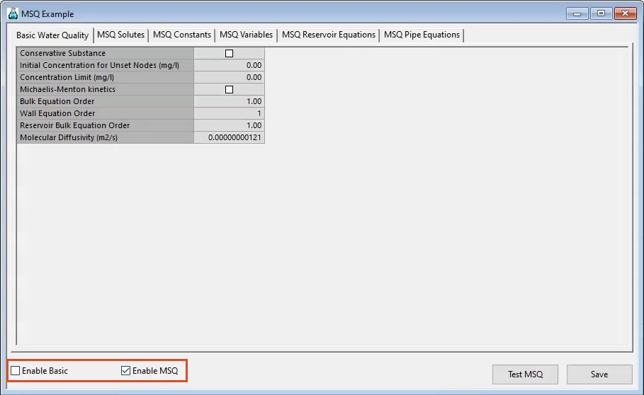
In the MSQ Example dialog box, Basic Water Quality tab, Enable Basic is deselected and Enable MSQ is selected.

  1. Click the MSQ Solutes tab.
  2. In the first row, set the WQ Solute ID as A.

Solute IDs are used in property sheets and in the results, and must be unique within this grid.

  1. In the same row, set the WQ Solute Description as A.
  2. In the second row, set the WQ Solute ID as B.
  3. Set WQ Solute Description as B.
  4. Set the third WQ Solute ID as C.
  5. Set WQ Solute Description as C.
  6. For all three rows, from the Solute Type drop-down, select Bulk (Dissolved).

This specifies that the solute is present in the bulk liquid, rather than on the pipe walls.
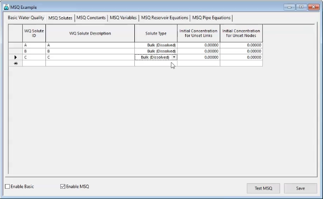
The MSQ Example dialog box, MSQ Solutes tab, with Bulk (Dissolved) selected in the Solute Type column for solutes A, B and C.

  1. For all three rows, leave the Initial Concentration for Unset Links and Nodes set to zero.
  2. Select the MSQ Constants tab.

Optional constants IDs can be defined to make equations easier to read. The constant IDs are replaced by the associated numerical values when the engine acts upon the equations.

  1. In the first row, specify the WQ Constant ID as Mass A.
  2. Set the WQ Constant Description as Molecular Mass A.
  3. Set the WQ Constant Value as 1.
  4. In the second row, set the WQ Constant ID as Mass B.
  5. Set the WQ Constant Description as Molecular Mass B.
  6. Set the WQ Constant Value as 1.
  7. In the third row, specify the WQ Constant ID as Mass C.
  8. Set the WQ Constant Description as Molecular Mass C.
  9. Set the WQ Constant Value as 2.

In the MSQ Example dialog box, MSQ Constants tab, three constant IDs, descriptions, and values are entered in the table.

  1. Select the MSQ Variables tab, which defines the variable IDs.
  2. In a text editor, open the MSQ_Variable.txt file for this exercise.
  3. Copy the script provided.
  4. In the MSQ Example dialog box, on the MSQ Variables tab, paste the script into the text box.

In the MSQ Example dialog box, the MSQ Variables tab with the script from MSQ_Variable.txt copied and pasted into the text box.

  1. Select the MSQ Reservoir Equations tab, which defines how solutes change over time within reservoirs.
  2. Copy and paste the script provided in the MSQ_Reservoir_Equations.txt file.
  3. Select the MSQ Pipe Equations tab, which defines how solutes change over time in pipes.
  4. Copy and paste the script provided in the MSQ_Pipe_Equations.txt file.
  5. Click Test MSQ to ensure that there are no errors.
  6. Click Save.

Now that the MSQ model has been set up, the next step is to dose the network with the contaminants.

Was this information helpful?