Controlling LOD with detail and surrounds surfaces
Any referenced datasets can be downloaded from "Module downloads" in the module overview.
Controlling LOD with detail and surrounds surfaces - Exercise
Task 1: Create surface from DEM
The DEM file is the result of filtering the classified point cloud to create a grid file of only ground surface points, which will save a lot of editing and clean-up time to get a good representation of the existing topographic features of the large project site.
- Open drawing named Surrounds Surface Start.dwg, found in the course dataset.
- On the Prospector Tab, right-click on the Surfaces collection and select Create Surface from DEM.
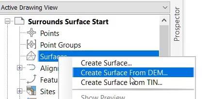
- Browse to and select Surrounds Ground Class Only.tif. Make sure GEOTIF *.tif is the file type.
Task 2: Review surface properties
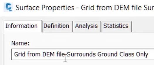
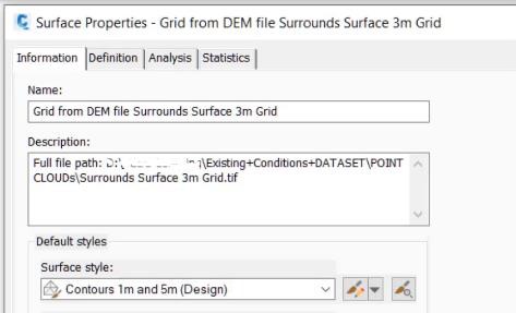
- After the surface is created, review the Surface Properties and note that the Name of the surface is derived from the name of the data file with a prefix of Grid from DEM.
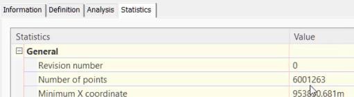
- Note the number of points in the surface is about 6 million points.
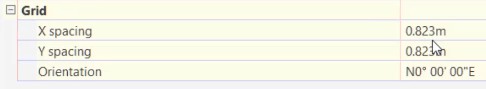
- Note the Grid spacing is 0.823 meters.
- Note that the LEVELOFDETAIL is turned on so that all contours may not be displayed in zoomed out views.
Task 3: Export DEM surface
The grid spacing of the original surface created from point cloud data has a 0.823 meter spacing which is too detailed for the purpose of a large surrounds surface and the number of points exceeds the maximum point limit of 1 million points. Exporting a new DEM from this surface will enable the grid spacing to be set at a much larger spacing which will have a benefit of also reducing the number of surface points to a value well beneath the maximum limit.
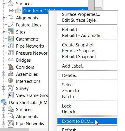
- Right-click on the new surface in the Surfaces collection on the Prospector tab, and select Export to DEM.
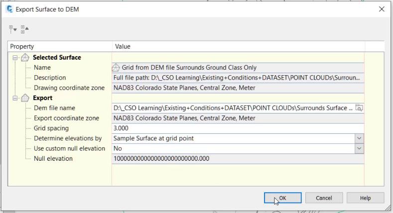
- In the Export Surface to DEM dialog box, enter the name of the new surface after browsing to the folder that you want to store it in. In this example it is being saved to the POINT CLOUDs folder of the dataset. Name the file Surrounds Surface 3m Grid.
- Change the Grid spacing value to 3.00.
- Select Sample Surface at grid point for the Determine elevations by value.
- Select OK to create the DEM file.
Task 4: Import the new DEM file to create a new grid surface
A new DEM surface to be used as the surrounds surface is created from the newly generated GeoTif file. This surface will be much smaller in point number size because of the 3.0 meter grid spacing, however the surface remains with enough resolution to be used for the surrounds surface purposes.
- Repeat the steps 2 and 3 in Task 1, use the newly created 3 meter GeoTif file.
- Note the difference in files sizes between the original tif file and this new reduced data tif file.

Task 5: Review surface properties
Repeat steps 1 and 2 in Task 2 to see that the number of points in the new surface abject named: Grid from DEM file Surrounds Surface 3m Grid is just over 450 thousand points, which is below the 1 million point maximum.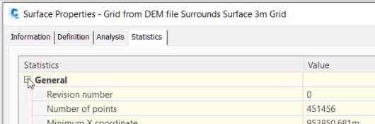
Task 6: Compare surfaces
- Change the style of the Grid from DEM file Surrounds Surface 3m Grid surface to Contours 1m and 5m (Design).
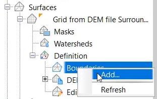
To save processing time and limit the data computations, add boundaries to both surfaces. Use the blue rectangle entities as the boundaries. To do this: - Expand the surface collection and the individual surfaces to see the Definition collection.
- In the Definition collection, right-click on Boundaries and select Add.
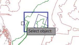
- Verify that the Type is Outer in the Add Boundaries dialog box, click on OK, and select on the larger blue rectangle.
- Repeat steps 2, 3, and 4 directly above. This places a boundary on both surfaces and will save processing time.
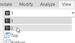
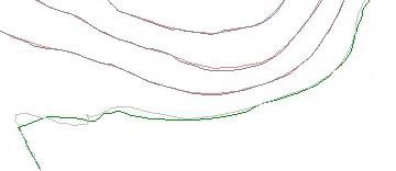
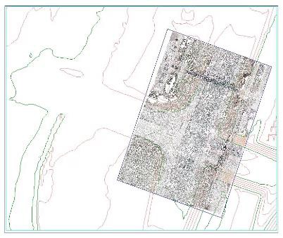
- On the View ribbon tab select Named View 2.
- Zoom and pan around to see the differences between the original contours in grey and the new simplified data contours in green and red.
Task 7: Create detail TIN surface
Using classified point cloud data to build surface usually results in a Grid type surface which is limited to one million points. If a TIN surface is created then the maximum number can be increased to 1.5 to 2 million points. An additional benefit to using a TIN surface is the additional edits that can be made to further refine the definition.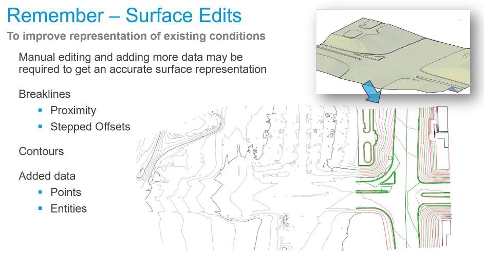
- Delete the original DEM surface: Grid from DEM file Surrounds Surface. This surface has too many points and if this drawing is saved it will generate overflow .GRD files. The overflow flies should be avoided as they create additional reference files that must remain linked to the drawing file. To delete the surface, select the surface in the Surfaces collection and click on Delete in right-click pop-up menu.
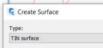
- On the Prospector Tab, right-click on the Surfaces collection and select Create Surface.
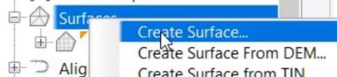
- Verify in the Create Surface dialog box that the Type is TIN Surface.
- Name the surface Intersection Detail and use the Contours 1m and 5m (Background) style.
- Select OK.
- On the Prospector tab, expand the Surface collection and the Intersection Detail surface Definitions. Right-click on DEM Files and select Add.
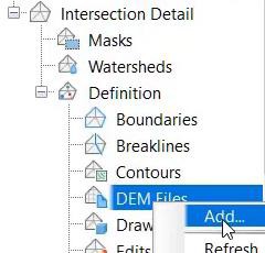
- Browse to and select Intersection and Bus Stop Ground Only.tif.
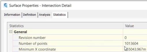
Task 8: Review surface properties
On the Statistics tab note the number of points is just over 1 million. And because this is a TIN surface now additional edits, such as adding breaklines, can be made to refine the definition.
In this drawing we have two surfaces: one representing the large area of surrounds and the other representing the details needed in an area of construction, modification, or rehabilitation. In both cases it is important to limit the number of points so that overflow: .MMS or .GRD files are not generated.
You do not need to save this Civil 3D drawing.